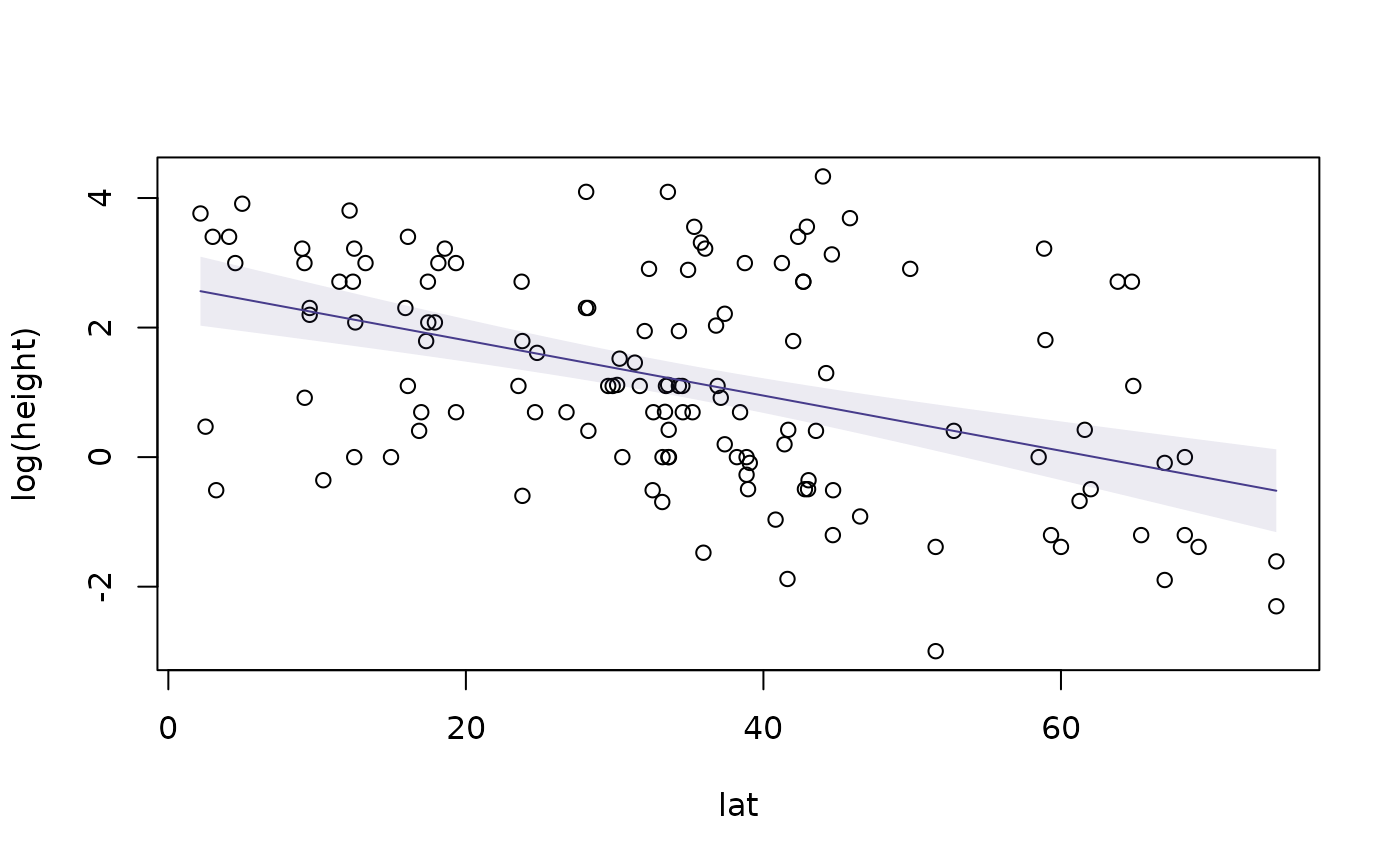
addSmooth Add a smoother to a plot, with pointwise confidence band

Adds a smoother to a plot of y against x, and a confidence band around the smoother with pointwise coverage (not global, unlike plotenvelope). The smoother is constructed using gam and confidence bands use Wald intervals, extracting the standard error from predict.gam.

Usage

addSmooth(
  x,
  y,
  conf.level = 0.05,
  line.col = "slateblue4",
  envelope.col = adjustcolor(line.col, alpha.f = 0.1),
  ...
)

Arguments

x: is the x co-ordinates for the plot, e.g. the fitted values in a plot of residuals vs fitted values.
y: is the y co-ordinates for the plot
conf.level: the confidence level to use in constructing the confidence band around the smoother.
line.col: color of smoother. Defaults to "slateblue4".
envelope.col: color of the global envelope around the expected trend. All data points should always stay within this envelope (and will for a proportion conf.level of datasets satisfying model assumptions). If a smoother has been used on the residual vs fits or scale-location plot, the envelope is constructed around the smoother, that is, the smoother should always stay within the envelope.
...: further arguments sent through to lines and polygon.

Value

A smoother is added to the existing plot, with confidence band. In addition, a data frame is invisibly returned with the following components:

X: The values of x at which the smoother is evaluated.
Yhat: Values of the smoother used to predict y, for each value of x.
Yhi: The upper bound on the confidence band, for each value of x.
Ylo: The lower bound on the global envelope, for each value of x.

Details

A challenge when interpreting diagnostic plots is understanding the extent to which deviations from the expected pattern could be due to random noise (sampling variation) rather than actual assumption violations. This function is intended to assess this, by simulating multiple realizations of residuals (and fitted values) in situations where assumptions are satisfied, and plotting a global simulation envelope around these at level conf.level.

This function adds a smoother to a plot of y against x using gam, and a confidence band around the smoother with pointwise coverage (not global, unlike plotenvelope) using Wald intervals that take the standard error of predicted values from predict.gam.

When constructing a plot to diagnose model fit, plotenvelope is preferred, because this constructs simulation envelopes globally, simplifying interpretation, and tends to give more accurate envelopes, via simulation. This function is intended to fit trends to data for descriptive purposes, but it could be used (with caution) to diagnose model fit in residual plots in situations where plotenvelope is unavailable.

References

Warton DI (2022) Eco-Stats - Data Analysis in Ecology, from t-tests to multivariate abundances. Springer, ISBN 978-3-030-88442-0

Author

David Warton <david.warton@unsw.edu.au>

Examples

data(globalPlants)
plot(log(height)~lat,data=globalPlants)
with(globalPlants, addSmooth(lat,log(height)) )